Can anybody provide me with a simplistic breakdown of what each of these are and how they differ?
I’ve read the Schweser notes but it is very wordy so if possible I would like to have a different explanation if possible please!
Can anybody provide me with a simplistic breakdown of what each of these are and how they differ?
I’ve read the Schweser notes but it is very wordy so if possible I would like to have a different explanation if possible please!
Minimum-Variance Frontier : The set of all risky portfolios having minimum risk (standard deviation of returns) for a given level of expected return. The horizontal axis is the standard deviation of returns, and the vertical axis is the expected return. The risk-free asset is not included in the portfolios considered for the minimum-variance frontier. The portfolio furthest to the left on the minimum-variance frontier is called the global minimum-variance portfolio, and any portfolio on the minimum-variance frontier is called an optimal portfolio.
Efficient Frontier : The portion of the minimum variance frontier that lies above (and to the right of) the global minimum-variance portfolio: the upper half of the minimum-variance frontier. This is the set of all risky portfolios having maximum return for a given level of risk (standard deviation of returns). The horizontal axis is standard deviation of returns, and the vertical axis is expected return. Any portfolio on the efficient frontier is called an efficient portfolio. All efficient portfolios are optimal, but not all optimal portfolios are efficient.
CAL : A line (technically, if you’re a geometer, a ray) running from the risk-free asset through a given (risky) asset (a single stock, a portfolio, whatever) and on to infinity. The horizontal axis is the standard deviation of returns, and the vertical axis is the expected return. The slope of the line is the Sharpe ratio of the given asset.
CML : The CAL with the largest Sharpe ratio. This line is tangent to the efficient frontier, and the tangency point is called the market portfolio. Thus, the slope of the CML is the Sharpe ratio of the market portfolio. The horizontal axis is the standard deviation of returns, and the vertical axis is the expected return.
SML : The line running from the risk-free asset through the market portfolio and on to infinity. The horizontal axis is the beta of the portfolio, and the vertical axis is the expected return. The slope of the SML is the market risk premium: the expected return of the market portfolio minus the risk-free rate.
Perfect.
Also great explanation regarding optimal/efficient portfolios. Thanks.
My pleasure.
The tagency point is also called the optimal riskly portfolio.
Without the “l”.


For the CAL, for level 1 is it essentially useless as we assume homogenous expectations and therefore it equals the CML?
No.
A CAL doesn’t have to go through the market portfolio. A CAL goes through a specified risky portfolio.
Dear magician
Your posts are helpful. Thanks!
Now at level 3 and it says in reading 31 schweser that “a superior manager will have a higher Sharpe than the market and a steeper CAL than the CML”
Does that not contradict what you say when you say that the steepest cal will be the cml?
It depends on a lot of assumptions.
If the market portfolio really is the market portfolio – with every investible asset (stocks, bonds, derivatives, wine, Ferraris, paintings, baseball cards, whatever) included – then the statement is clearly false: the manager can’t invest in anything that isn’t included in the market portfolio by definition.
However, if the market portfolio is just some handy proxy for the market – say, the S&P 500 index – then it’s certainly possible to have a higher Sharpe ratio than the market’s Sharpe ratio.
"efficient portfolio. All efficient portfolios are optimal, but not all optimal portfolios are efficient" Could you clarify the difference between optimal versus efficient?
An optimal portfolio has the minimum amount of variance for a given expected return. In the image below, L and M are both optimal since for their given level of expected return they have the smallest possible variance.
Efficiency on the other hand looks at the maximum amount of expected return for a given level of risk. So L and M have the same amount of risk, but L is clearly more efficient since it has a higher level of expected return for the same variance.
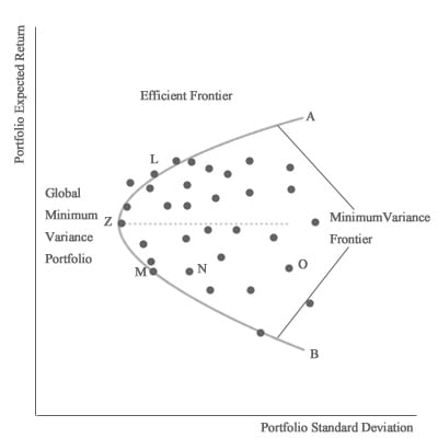
Source for image: https://ift.world/booklets/5-2-minimum-variance-portfolios/
Your explanation is good, but the picture is silly: I see three portfolios (L being one of them) that are to the left of the efficient frontier. That’s impossible.